Building a machine-learning pipeline with scikit-learn and Qt - Part II

Alexandre Pinto

2017-09-02

machine-learning, python, qt5, scikit-learn

In order to run experiments, we need a data. This dataset was the same used in a research study, consisting of data payments gathered during October, 2005, from a bank in Taiwan, using the credit card holders from that bank as the study targets.

In the first part we talked about the process of machine learning. This post will discuss data gathering and the dataset.

Data Gathering

The first step is to collect the training and testing data such as sufficient and representative data. This usually implies tasks such as:

Data Integration - The initial data might come from different sources, with different formats or duplicated data. This step is important to create a single repository of data.
Data Balancing - As is often the case with real data, the data is usually not uniformly distributed across the different classes. Consequently, the trained models tend to predict new data with the majority class. Techniques to artificially balance the data might be employed here, such as reducing (Undersampling) / increasing (Oversampling) the number of instances from the majority /minority classes. An other alternative might be performing a stratified sampling in order to keep a significant number of instances in each class.
Cleaning - The quality of the data is important. Sometimes the data will have missing attributes or useless values. However, redundant or noisy data are important issues to be addressed, such as instances with very similar feature values, attributes easily deducted from others or outliers.

The dataset

Each sample of the dataset contains 23 variables and a predictive binary label (Defaul payment: Yes = 1, No = 0). These 23 features are described as follows:

X1: Amount of the given credit
X2: Gender (1 = male; 2 = female)
X3: Education (1 = graduate school; 2 = university; 3 = high school; 4 = others).
X4: Marital status (1 = married; 2 = single; 3 = others)
X5: Age (age in years)
X6-X11: History of past payment (X6 = the repayment status in September, 2005 ; . . .; X11 = the repayment status in April, 2005), where x = -1 = pay duly and x = 1,2,3, ..9 = payment delay for x months
X12-X17: Amount of bill statement
X18–X23: Amount of previous payment

The GUI

The resulting application has a tab designed to show a quick description of the loaded dataset, that is, the description of the features, the cardinality of each class and some statistical measures of each feature:

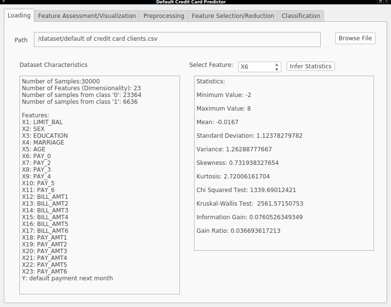
For the design of the interface, the Qt Designer is a great tool to quickly generate our GUI. This tool generates a .xml file describing the UI, which is then used to generate a python module which we can import and use to load the main interface.

The extraction of statistical metrics is useful to get a quick overview of how our data is distributed. We will talk about these metrics later in detail.

Part III will provide an overview of feature assessment and visualization.