Speeding up python programs with Numba and Numpy
When Python is not enough
The Python programming language is a great tool for almost any kind of rapid prototyping and quick development. It has great features such as its high level nature, a syntax with almost human-level readability . Besides, it is cross platform, with a a diverse standard library and it is multi-paradigm, giving a lot of freedom to the programmer which can use different programming paradigms such as object-oriented, functional or procedural as he sees fit. However, sometimes some portion of our system has high performance requirements and thus the speed that Python offers might not be sufficient. So, how can we boost performance without leaving the realm of Python (using for example compiled languages such as C/C++ or JIT/compiled such as JAVA) and when all of our optimizations are not enough anymore ?
A possible solution, among others, is to make use of Numba, a runtime compiler that translates Python code to native instructions, while letting us use the concise and expressiveness power of Python and also achieve native code speed.
Whats is Numba ?
Numba is a library that performs JIT compilation, that is, translates pure python code to optimized machine code at runtime, using the LLVM industry-standard compiler. It is also able to automatically parallelize loops and run them on multiple cores. Numba is cross-platform since it works on different operative systems (Linux, Windows, OSX) and different architectures (x86, x86_64, ppc64le, etc). It is also able to run the same code on a GPU (NVIDIA CUDA or AMD ROC) and is compatible with Python 2.7 and 3.4-3.7. Overall, the most impressive feature is its simplicity of use since we only need a few decorators to leverage the full power of JIT optimizations.
Numba modes and the @jit decorator
The most important instruction is the @jit decorator. It is this decorator that instructs the compiler which mode to run and with what configurations . Under the hood, the generated bytecode of our decorated functions combined with the arguments that we specify in the decorator, such as the type of the input arguments, are analysed, optimized and finally compiled with the LLVM, generating specially tailored native machine instructions for the CPU currently in use. This compiled version is then reused for each function call.
There are two important modes: nopython and object. The nopython completely avoids the python interpreter and translates the full code to native instructions that can be run without the help of Python . However, if for some reason, that mode is not available (for example, when using unsupported Python features or external libraries) the compilation will fall back to the object mode, where it uses the Python interpreter when it is unable to compile some code . Naturally, the nopython mode is the one who offers the best performance gains.
High-level architecture of Numba
The Numba translation process can be translated in a set of important steps ranging from the Bytecode analysis to the final machine code generation. The picture bellow illustrates this process, where the green boxes correspond to the frontend of the Numba compiler and the blue boxes belong to the backend.
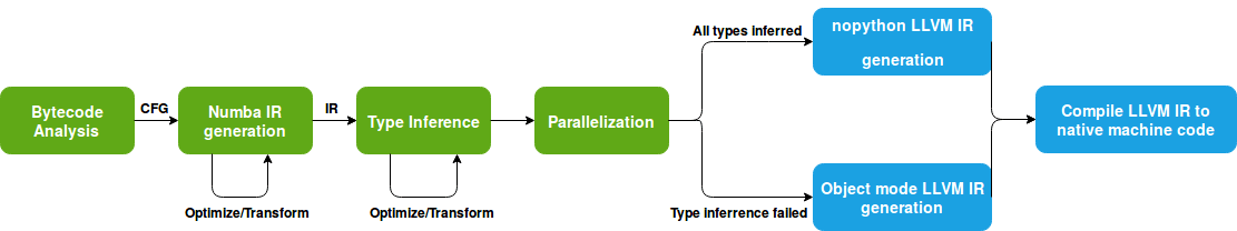
The Numba compiler starts by doing an extensive analysis on the byecode of the desired function(s). This step produces a graph describing the possible flow of executions, called control flow graph (CFG). Based on this graph an analysis on the variable lifetimes are calculated. With these steps finished, the compiler starts translating the bytecode into an intermediate representation (IR) where Numba will perform further optimizations and transformations. Afterwards, type inference, one of the most important steps, is performed. In this step, the compiler will try to infer the type of all variables. Furthermore, if the parallel setting is enabled, the IR code will be transformed to an equivalent parallel version.
If all types are successfully inferred, the Numba IR code is then translated into an efficient LLVM IR code, completely avoiding the Python runtime. However, if the type inference process fails, the LLVM generated code will be slower since it still needs to deal with calls to Python C API. Finally, the LLVM IR code is compiled into native instructions by the LLVM JIT compiler. This optimized machined code is then loaded into memory and reused across multiple calls to the same function(s), making it hundreds of times faster than pure Python.
For debugging purposes, Numba also offers a set of flags that can be enabled in order to see the generated output of the different stages.
1 | import os |
Speeding numerical computations: An example
The best use case where we can make use of the Numba library is when we have to do intensive numerical computations. As an example, let's compute the softmax function on a set of 2^16 (65536) random numbers. The softmax function, useful to convert a set of real values into probabilities and commonly used as the last layer in neural networks architectures, is defined as:
\[ \sigma(z_j) = { e^{z_j} \over \sum_{k=1}^{K} e^{z_k} } \]
The following code show two different implementations of this function, a pure python approach (softmax_python) and an optimized version making using of numpy and numba (softmax_optimized):
1 | import time |
The result of the above script will be something similar to:
1 | > python softmax.py |
These results clearly shows the performance gains obtained when converting our code to something that Numba understands well.
In the softmax_optimized function, there is already the Numba annotation that leverages the full power of JIT optimizations. In fact, under the hood the following bytecode will be analysed, optimized and compiled to native instructions:
1 | > python |
We can provide more information about the expected input and output types through the signature. In the example above, the signature "f8[:](f8[:])" is used to specify that the function accepts an array of double precision floats and returns another array of 64-bit floats.
The signature could also use the explicit type names: "float64[:](float64[:])". The general form is type(type, type, ...) which resembles a typical function where argument names are replaced by their types and the function name is replaced by its return type. Numba accepts many different types, which are described bellow:
| Type name(s) | Type short name | Description |
|---|---|---|
| boolean | b1 | represented as a byte |
| uint8, byte | u1 | 8-bit unsigned byte |
| uint16 | u2 | 16-bit unsigned integer |
| uint32 | u4 | 32-bit unsigned integer |
| uint64 | u8 | 64-bit unsigned integer |
| int8, char | i1 | 8-bit signed byte |
| int16 | i2 | 16-bit signed integer |
| int32 | i4 | 32-bit signed integer |
| int64 | i8 | 64-bit signed integer |
| intc | – | C |
| uintc | – | C |
| intp | – | pointer-sized integer |
| uintp | – | pointer-sized unsigned integer |
| float32 | f4 | single-precision floating-point number |
| float64, double | f8 | double-precision floating-point number |
| complex64 | c8 | single-precision complex number |
| complex128 | c16 | double-precision complex number |
These annotations are easily extended to array forms using [:] , [:, :] or [:, :, :] for 1, 2 and 3 dimensions, respectively.
Final words
Python is a great tool. However, it has some limitations which can be surpassed with the right strategy, making it competitive, in terms of performance, to other compiled languages. Although this post focused on the Numba library, there are other good options (which deserve their own dedicated blog post). Numba also offers other great features not explored here such as integration with NVIDIA CUDA/AMD ROC GPUs, interfacing with C functions and Ahead-of-Time compilation (AOT). Finally, the example source code can be found here.