Building a machine-learning pipeline with scikit-learn and Qt - Part VI
In the learning phase a set of examples are shown to the classifier, with class labels (supervised learning) or without them (unsupervised learning). As a result, the classifier is then able to categorize, with a certain accuracy, new unseen data. Experimental evaluation is also an important step to assess the effectiveness of a classifier, i.e, the quality of the decisions made by a predictive model on unseen data. This post is a follow up from the previous post and describes some classical and well-known learning methods available and how to evaluate their performance.
Classifiers
Some common learning algorithms are described bellow:
Minimum Distance Classifier - Minimum Distance Classifiers are template matching system where unseen feature vectors are matched against template prototypes (vectors) representing the classes. This matching usually involves computing the matching error between both feature vectors using for example the euclidean distance as the error metric. This matching distance can simply be stated as: \[ || x - m_k|| \] where x is the unseen feature vector and mk is the feature prototype for class k, usually consisting in a feature vector with feature mean values obtained during the training phase. After k tests are performed, the class belonging to the prototype with the minimum distance is chosen.
k-Nearest Neighbor (kNN) - The kNN is a simple and fast unsupervised algorithm that classifies unknown instances based on the majority class from k neighbors. This method starts by constructing a distance matrix between the training samples and the new test sample and chooses the nearest k neighbors. Afterwards, the majority label from these neighbors is assigned to the new data. For two-class problems, k is usually an odd number to prevent ties.
Naive Bayes - The Naive Bayes Classifier is a simple supervised probabilistic model based on the Bayes’ theorem. The posterior probabilities are computed for each class wj and the class with largest outcome is chosen to classify the feature vector x. To achieve this result, the likelihood, prior and evidence probabilities must be calculated, as shown below: \[ posterior \, probability = { likelihood \times prior \; probability \over evidence} \] \[ P(w_j | x) = { p(x|w_j) \times P(w_j) \over p(x) } \] The main difficulty is to compute the likelihoods p(x|ωj) since the other factors are obtained from the data. P(ωj) are the prior probabilities and p(x) is a normalization factor which is sometimes omitted. Assuming independence of the features, the likelihoods can be obtained as shown bellow: \[ P(x | w_j) = { \prod P(x_k | w_j) } \] This simplification allows to compute the class conditional probabilities for each feature separately, reducing complexity and computational costs.
Support Vector Machines (SVM) - Support vector machines are optimization methods for binary classification tasks that map the features to a higher dimensional space where an optimal linear hyperplane that separates the existing classes exists. The decision boundary is chosen with the help of some training examples, called the support vectors, that have the widest separation between them and help maximizing the margin between the boundaries of the different classes. The decision surface is in the “middle” of these vectors. During the training phase, the coefficient vector w and the constant b that define the separating hyperplane are searched such that the following error function is minimized: \[ minimize: {1 \over 2} ||w||^2 + C \sum ξ_i \] \[ s.t. \quad y_i(φ(x_i) + b) \geq 1 - ξ_i \] where C is an arbitrary constant and ξ are slack variables used to penalize misclassified instances that increase with the distance from the margin. If C is large, the penalty for misclassification is greater. The vectors xi are the training instances. This method makes use of a kernel function φ used to transform the input vectors into higher dimensional vectors. New instances are then classified according to which ”side” of the hyperplane they are located.
Decision Tree - Decision Trees are supervised methods that learn rules based on the training data to classify new instances. The built trees are simple to understand and visualize. During training, each node of the tree is recursively split by the feature that provides, for example, the best information gain.
Random Forest - Random forests are ensemble methods, i.e., they take into consideration the prediction of several classifiers in order to improve the accuracy and robustness of the prediction results. In the case of random forests, they train a set of random trees with bootstrapped samples (samples drawn with replacement) from the original training data. Each tree is grown by selecting m random features from the d features and recursively splitting the data by the best splits. The classification of new data is achieved by a majority vote.
Each classifier has its own advantages and disadvantages and the right technique should be chosen according to the requirements of the problem-at-hand.
Evaluation Metrics
In classification tasks, predictions made by a classifier are either considered Positive or False (under some category) and the expected judgments are called True or False (again, under a certain category). Common metrics are:
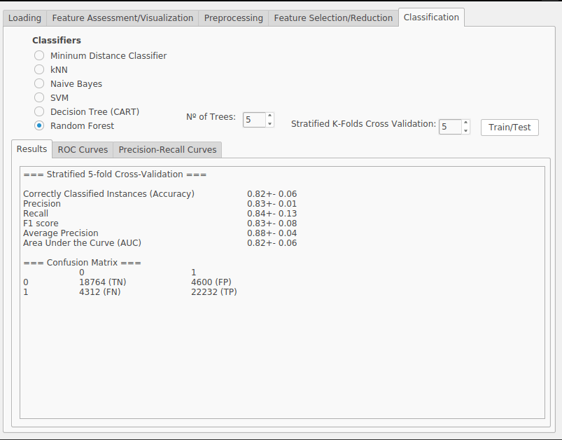
Accuracy - This measure provides a proportion of correctly classified instances and correctly rejected instances (True Positives and True Negatives) among the whole dataset. \[ Acc = {TP + TN \over TP + TN + FP + FN}\]
Precision - This measure provides a proportion of correctly classified instances (True Positives) among all the positive identified instances (True Positives and False Positives). \[ P = {TP \over TP + FP }\]
Recall - This measure, sometimes called sensitivity, provides a proportion of correctly classified instances (True Positives) among the positive instances that were and should have been correctly identified, i.e., the whole positive part of the dataset (True Positives and False Negatives). \[ R = {TP \over TP + FN }\]
F-measure - This measure combines precision and recall and provides a balance between them. It is computed as the harmonic mean between the two metrics providing the same weight for both. \[ F_1 = {2 \times P \times R \over P + R }\]
Stratified K-fold Cross Validation - A popular technique to evaluate the performance of the system is to split the data into training and testing sets, using the later to estimate the true generalization performance of the classifier. However, this may bring some issues such as the trade-offs between the percentage splits or the representativity of the test set. A popular accepted approach is to split the entire dataset into k representative partitions, using k − 1 of these partitions for training and the remaining one for testing. This process is then repeated k times, (each time using a different test partition) and the results averaged.
Visualizing the performance
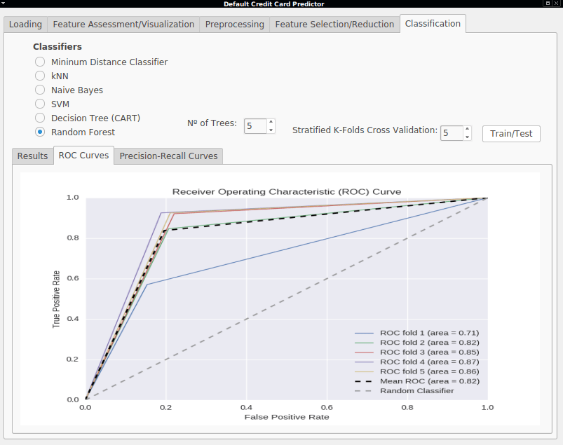
- Receiver Operating Characteristics (ROC) - ROC curves are useful graphs to visualize the performance of binary classifiers. They are useful to compare the rates at which the classifier is making correct predictions (True Positive Rate plotted on the Y axis) against the rate of false alarms (False Positive Rate plotted on the X axis). Important points in this graph are the lower left point (0,0), representing a classifier that never classify positive instances, neither having False Positives or True Positives. On the other hand, the upper right point (1,1) represents a classifier that classifies every instance as positive, disregarding if it is a false positive or not. Finally, the point (0,1) represents the perfect classifier, where every instance was correctly classified. The area bellow the ROC curve is called Area Under the Curve (AUC) and is also a good evaluation measure. A perfect classifier would have an AUC of 1.0 while a random classifier would only have 0.5.
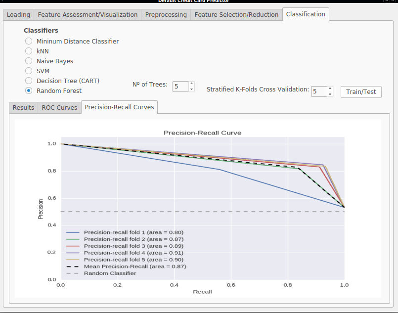
- Precision-Recall Curves (PR) - The Precision-Recall Curve plots the trade-off between the precision and recall achieved by a classifier, by showing the recall on the X axis and precision on the Y axis. An important point in this graph is the upper right point (1,1) which represents the ideal classifier having maximum precision and recall. Figure 2.4 shows three hypothetical classifiers and the areas of good and bad performance, which are above or below the line defined by a random classifier. The area bellow the PR curve is called Average Precision (AP) and is also a good measure. A perfect classifier would have an Average Precision of 1.0 while a random classifier would only have 0.5.
In this series of posts, a machine learning application was presented, showing a typical pipeline with the following steps:
Dataset Loading
Feature Assessment where the distribution of features are inspected and visualized
Preprocessing where data transformations are applied and issues such as dataset balancing are addressed.
Feature Selection methods where features with he most discriminative power are selected
Classifications performed by predictive models where their performance is evaluated using ROC curves, Precision-Recall Curves and generic metrics such as Accuracy, Precision, Recall and F1 measures.
The machine learning method is an iterative process, where one needs to go back and forth, setting different parameters, and different methods in order to see which combination works best and provides the best results. You can checkout this application and try it for yourself. The source code is available in this repository.